K1GGI FMT METHODOLOGY

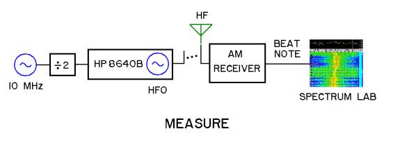
The measurement method is to heterodyne a precise local oscillator (HFO) with the unknown FMT signal, then detect and measure the AF beat note with high precision. The implementation takes advantage of some gear I have on hand.

LOCAL REFERENCE OSCILLATOR

The method starts with having a high-stability Local Oscillator (LO) as a reference. The best reference I have is the 10MHz precision crystal oscillator in a HP 8594E spectrum analyzer. This oscillator is spec’d for 1e-7/year aging and 1e-8 from 0 to 55ºC.

HFO SIGNAL GENERATOR

The HP 8640B signal generator can lock its tuned-cavity oscillator to a reference, such that its output is a rational multiple of that reference, with 100Hz granularity at common FMT frequencies. The key property is that the ratio is exact, and introduces no error.

RECEIVER

The receiver doesn’t have to be anything special as long as it can tune to the FMT in AM mode and detect the heterodyne.

BEAT NOTE

The beat note is fed to a computer sound card and recorded directly as a 44.1kHz wav file for later analysis with Spectrum Lab software. I use a fairly high resolution fft (decimate 64, length 32768).

CALCULATION

The 8640B serves as the HFO. It gets tuned and locked to several hundred Hz below the unknown FMT carrier. A short wire on the output of the generator is enough for it to be picked up and produce a beat with the unknown signal in the am receiver. The unknown is then f_x = f_HFO + f_beat.

ACCURACY

Results depend on accurately knowing the HFO and beat frequencies. The HFO frequency is strictly proportional to the LO frequency; so if the LO is actually 10MHz × k, then f_HFO = f_set × k, where f_set is what the 8640 is set to. The prime calibration task is to determine the value of k to high accuracy.

The apparent f_beat depends on sound card sample rate, which I calibrate using a tone derived from the accurate LO crystal. The sound-card contribution to beat-note measurement error ends up being in the sub-millihertz range.

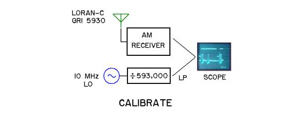
LO REFERENCE CALIBRATION

The LO calibration utilizes transmissions of the Loran-C navigation system as a reference. Loran transmissions are pulse-modulated 100kHz carriers with cesium-referenced timing. Loran-C transmissions were being used as high-accuracy time/frequency references before GPS was widely deployed.

Nantucket Island, 30 miles away, is the site of the transmitter for the X secondaries of two Loran-C chains, GRI 5930 and 9960. The strong stable signal is an excellent off-the-air reference here.

Complete Loran-disciplined frequency standards are manufactured and available, but for the purpose of calibrating an oscillator in the ham shack, I take a hands-on approach using a general-coverage receiver along with a bit of homebrewing.

The 5930 GRI transmission is a burst of pulses that repeat with a 59,300 microsecond period. Dividing the 10MHz local oscillator by 593,000 yields a 59,300 microsecond pulse (Local Pulse, LP) that can be compared with the Loran transmission, as shown here.

The next photo shows the LP and the am-detected Loran waveform lined up on an oscilloscope set for a 10ms/div time scale. The scope is triggered on the LP. This scale shows a complete period of the 5930 GRI, which occupies 5.93 divisions on the graticule. (This photo has been retouched to overcome shutter and sweepspeed issues.)

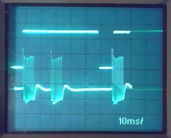
Since Nantucket is transmitting at two rates, the live scope trace shows the 9960 bursts popping up all over the place, while the 5930 bursts appear stationary. This photo happened to capture one 9960 burst. Nantucket is so strong here that it is difficult to pick out the low-level bursts from the distant master or the other secondaries, but they are there.

The next photo expands the timescale to show the leading pulse of the Nantucket 5930-X GRI lined up with the rising edge of the 59,300µs LP. The traces are positioned so the ‘corner’ of the LP just kisses the slope of the Loran pulse. This makes it easy to see small changes in the relationship over time.

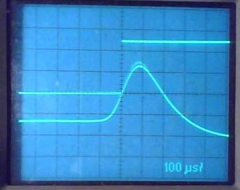
If the 10MHz LO is as perfect as the Loran timing reference, there will be no drift seen on the scope. On this 100µs/div scale, a drift of 20µs (1/5 division) can be detected by eye. In one hour, 20µs is about 6 ppb (6e-9, .06Hz @ 10MHz), and this is a ‘quick’ way to make a coarse estimate of the LO accuracy. Longer observations will give better numbers. For example, if the drift is judged to be 100µs ±10µs over 24 hours, that corresponds to 1.16 ±0.12 ppb. If the Loran appears to drift to the right (coming progressively later), it means the LP is triggering the scope too soon, which in turn means the LO crystal is running fast.

LO ADJUSTMENT

As described above, a computed LO correction factor k can be used in the FMT calculations, and it isn’t necessary for the oscillator itself to be perfectly accurate, as long as it is stable and its error is known. However, there is some enjoyment and satisfaction to be had by using the drift measurements to adjust out the error.

The oscillator module in the 8594 has a multiturn adjustment trimmer, and its spec for initial achievable accuracy is 22 ppb. Much beyond this, the adjustment gets pretty touchy, due to end play and hysteresis. With patience and perseverance, I have managed to get accuracy to within a few ppb.

In my first session trying this, preparing for the November 2007 ARRL FMT, I found the LO was low by about 400ppb. This is not bad considering that this 8594E is about 10 years old. The aging would be 4e-8/yr, which compares favorably to the spec of 10e-8/yr.

THE HOMEBREW CONNECTION

The 8640B needs 5MHz to lock to, so the 10MHz LO needs to be divided by two. The scope needs the 59,300µs LP, which means dividing the LO by 593,000. The next photo shows how this is accomplished.

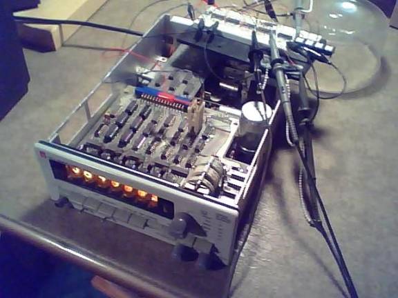
This is a GR 1192B counter, connected up with a few extra chips on a breadboard sitting at the back. The counter is locked to the LO and a few of its chips participate by doing some decades of division, while the breadboard does a final ¸593.

GETTING RESULTS

I check the LO and sample rate within a few days of the test.

The only skill involved during the test is to tune the receiver and set the 8640B, then start recording a wav file. I pick a comfortable beat note during the callup, and make sure to log the setting and confirm that it is really running below the target, so things will add up as expected.

Analyzing the file with Spectrum Lab is done at leisure. The results always have a befuddling amount of Doppler dispersion. I have been judging the screen images by eye to come up with a frequency. This part is not an exact science, but for whatever reason, it has gotten pretty close.